Pressure is defined as the ratio of force acting perpendicular and uniformly distributed per unit area.
Formula 1-3: Definition of pressure
-
p\quad\text{Pressure}\ [\text{Pa}] -
F\quad\text{Force}\ [\text{N}];\ 1\ \text{N}=1\ \text{kg}\ \text{m}\ \text{s}^{-2} -
A\quad\text{Area}\ [\text{m}^2]
In an enclosed vessel the gas particles perform thermal movements. In their interaction with the vessel wall, the atoms and molecules are subjected to a large number of collisions. Each collision exerts a force on the vessel wall. Where an enclosed gas is not exposed to outside influences, the numerous collisions that take place result in the same pressure occurring at any point within the vessel, no matter where and in what direction the measurement is carried out.
-
_grayscale(false)_format(webp)-2_news_article_1200x675.webp)
Figure 1.2: Definition of total pressure
_grayscale(false)_format(webp)-2_news_article_767x430.webp)
In practice, it is very rare that only one gas is available. Mixtures of different gases are much more common. Each single component of these gases will exert a specific pressure that can be measured independently of the other components. This pressure exerted by the various components is called partial pressure. In ideal gases, the partial pressures of the various components add up to the total pressure and do not interfere with each other. The sum of all partial pressures equals the total pressure.
-
_grayscale(false)_format(webp)-3_news_article_1200x675.webp)
Figure 1.3: Definition of partial pressure
_grayscale(false)_format(webp)-3_news_article_767x430.webp)
An example of a gas mixture is our ambient air. Its partial pressure composition is shown in Table 1.1. [3]
Gas type | Chem. Formula | Volume % | Partial pressure [hPa] |
|---|---|---|---|
Nitrogen | N2 | 78.09 | 780.9 |
Oxygen | O2 | 20.95 | 209.5 |
Water vapor | H2O | < 2.3 | < 23.3 |
Argon | Ar | 9.3·10 -1 | 9.3 |
Carbon dioxide | CO2 | 3.0·10-2 | 3.0·10-1 |
Neon | Ne | 1.8·10 -3 | 1.8·10-2 |
Hydrogen | H2 | < 1·10-3 | < 1·10-2 |
Helium | He | 5.0·10 -4 | 5.0·10-3 |
Methan | CH4 | 2.0·10-4 | 2.0·10-3 |
Krypton | Kr | 1.1·10 -4 | 1.1·10-3 |
Carbon monoxide | CO | < 1.6·10-5 | < 1.6·10-4 |
Xenon | Xe | 9.0·10 -6 | 9.0 . 10-5 |
Nitrous oxide | N2O | 5.0·10 -6 | 5.0·10-5 |
Ammonia | NH3 | 2.6·10-6 | 2.6·10-5 |
Ozone | O3 | 2.0·10-6 | 2.0·10-5 |
Hydrogen peroxide | H2O 2 | 4.0·10-8 | 4.0·10-7 |
Iodine | I2 | 3.5·10-9 | 3.5·10-8 |
Radon | Rn | 7.0·10 -18 | 7.0·10-17 |
Table 1.1: Composition of atmospheric air. The partial pressures indicated refer to 1,000 hPa. Note: The value indicated for water vapor is the saturated state at 293 K (20°C). The values for carbon dioxide and carbon monoxide fluctuate depending on the place and time. The indication for carbon monoxide is the peak value for a large city. Other sources refer to a natural hydrogen concentration of 5 · 10-5 % and a partial pressure of 5 · 10-4 hPa.
In space, depending on the proximity to galaxies, pressures of under 10-18 hPa prevail. On Earth, technically generated pressures of less than 10-16 hPa have been reported. The range of atmospheric pressure down to 10-16 hPa covers 19 decimal powers. Specifically adapted types of vacuum generation and measurement for the pressure range result in subdivisions of the various pressure ranges as shown in Table 1.2.
Pressure range | Pressure hPa | Pressure Pa | Number density per cm3 | Mean free path in m |
|---|---|---|---|---|
Atmospheric pressure | 1,013.25 | 101,325 | 2.7·1019 | 6.8·10-8 |
Low vacuum (LV) | 300…1 | 30,000…100 | 1019…1016 | 10-8…10-4 |
Medium vacuum (MV) | 1…10-3 | 100…10-1 | 1016 …1013 | 10-4…10-1 |
High vacuum (HV) | 10-3…10-8 | 10-1…10-6 | 1013…108 | 10-1…104 |
Ultra-high vacuum (UHV) | 10-8…10-11 | 10-6…10-9 | 108…105 | 104…107 |
Extremely high vacuum (XHV) | <10-11 | <10-9 | <105 | >107 |
Table 1.2: Pressure ranges in vacuum technology
The unit for measuring pressure is the pascal. This unit was named after the French mathematician, physicist, writer and philosopher Blaise Pascal (1623 – 1662). According to Formula 1-3, the SI unit pascal is composed of Pa = N m-2. The units mbar, torr and the units shown in Table 1.3 are common in practical use.
Pa | bar | hPa | µbar | Torr | micron | atm | at | mm WS | psi | psf | |
|---|---|---|---|---|---|---|---|---|---|---|---|
Pa | 1 | 1·10-5 | 1·10-2 | 10 | 7.5·10-3 | 7.5 | 9.87·10-6 | 1.02·10-5 | 0.102 | 1.45·10-4 | 2.09·10-2 |
bar | 1·105 | 1 | 1·103 | 1·106 | 750 | 7.5·105 | 0.987 | 1.02 | 1.02·104 | 14.5 | 2.09·103 |
hPa | 100 | 1·10-3 | 1 | 1,000 | 0.75 | 750 | 9.87·10-4 | 1.02·10-3 | 10.2 | 1.45·10-2 | 2.09 |
µbar | 0.1 | 1·10-6 | 1·10-3 | 1 | 7.5·10-4 | 0.75 | 9.87·10-7 | 1.02·10-6 | 1.02·10-6 | 1.45·10-5 | 2.09·10-3 |
Torr | 1.33·102 | 1.33·10-3 | 1.33 | 1,330 | 1 | 1,000 | 1.32·10-3 | 1.36·10-3 | 13.6 | 1.93·10-2 | 2.78 |
micron | 0.133 | 1.33·10-6 | 1.33·10-3 | 1.33 | 1·10-3 | 1 | 1.32·10-6 | 1.36·10-6 | 1.36·10-2 | 1.93·10-5 | 2.78·10-3 |
atm | 1.01·105 | 1.013 | 1,013 | 1.01·106 | 760 | 7.6·105 | 1 | 1.03 | 1.03·104 | 14.7 | 2.12·103 |
at | 9.81·104 | 0.981 | 981 | 9.81·105 | 735.6 | 7.36·105 | 0.968 | 1 | 1·10-4 | 14.2 | 2.04·103 |
mm WS | 9.81 | 9.81·10-5 | 9.81·10-2 | 98.1 | 7.36·10-2 | 73.6 | 9.68·10-5 | 1·10-4 | 1 | 1.42·10-3 | 0.204 |
psi | 6.89·103 | 6.89·10-2 | 68.9 | 6.89·104 | 51.71 | 5.17·104 | 6.8·10-2 | 7.02·10-2 | 702 | 1 | 144 |
psf | 47.8 | 4.78·10-4 | 0.478 | 478 | 0.359 | 359 | 4.72·10-4 | 4.87·10-4 | 4.87 | 6.94·10-3 | 1 |
Table 1.3: Conversion table for units of pressure
1.2.2 General gas equation
Each material consists of atoms or molecules. By definition, the amount of substance is indicated in moles. One mole of a material contains 6.022 · 1023 constituent particles (Avogadro constant. This is not a number but a physical magnitude with the unit mol-1). 1 mole is defined as the amount of substance of a system which consists of the same number of particles as the number of atoms contained in exactly 12 g of carbon of the nuclide 12C.Under normal conditions, i.e. a pressure of 101,325 Pa and a temperature of 273.15 K (equals 0°C), one mole of an ideal gas fills a volume of 22.414 liters.
As early as 1664, Robert Boyle studied the influence of pressure on a given amount of air. The results confirmed by Mariotte in experiments are summarized in the Boyle-Mariotte law:
Formula 1-4: Boyle-Mariotte law
Expressed in words the Boyle-Mariotte law states that the volume of a given quantity of gas at a constant temperature is inversely proportional to the pressure – the product of the pressure and volume is constant. Over a hundred years later, the temperature dependence of the volume of a quantity of gas was also identified: the volume of a given quantity of gas at a constant pressure is directly proportional to the absolute temperature or
Formula 1-5: Gay-Lussac’s law
Subjecting a given quantity of gas successively to a change in pressure and a change in temperature results in
\frac{p\cdot V}{T}=\mbox{const.} The quantity of material is determined by weighing. We can express the quantity of gas by the ratio of mass divided by the molar mass. The constant const. refers here to 1 mole of the gas in question, and it is referred to as the gas constant 𝑅. As a result, the state of an ideal gas can be described as follows as a function of pressure, temperature and volume:
Formula 1-6: General equation of state for ideal gases
- 𝑝 Pressure [Pa]
- 𝑉 Volume [m3]
- 𝑚 Mass [kg]
- 𝑀 Molar mass [kg kmol-1]
- 𝑅 General gas constant [kJ kmol-1 K-1]
- 𝑇 Absolute temperature [K]
The amount of substance 𝜈 can also be indicated as the number of molecules in relation to the Avogadro constant.
Formula 1-7: Equation of state for ideal gases I
- 𝑁 Number of particles
- 𝑁𝐴 Avogadro constant= 6.022 · 1023 [mol-1]
- 𝑘 Boltzmann constant= 1.381 · 10-23 [J K-1]
If both sides of the equation are now divided by the volume, then we obtain
Formula 1-8: Equation of state for ideal gases II
𝑛 Particle number density [m-3]
1.2.3 Molecular number density
As can be seen from Formula 1-7 and Formula 1-8 pressure is proportional to particle number density. Due to the high number of particles per unit of volume at standard conditions, it follows that at a pressure of 10-12 hPa, for example, 26,500 molecules per cm³ will still be present. This is why it is not possible to speak of a void, or nothingness, even under ultra-high vacuum. In space it is increasingly ineffective at extremely low pressures to express pressure in the unit Pascal, e. g. less than 10-18 hPa. These pressure ranges can be better expressed by the particle number density, e. g. < 104 molecules per cubic meter in interplanetary space.1.2.4 Thermal velocity
Gas molecules enclosed in a vessel collide entirely randomly with each other. Energy and impulses are transmitted in the process. As a result of this transmission, a distribution of velocity and/or kinetic energy occurs. The velocity distribution corresponds to a bell curve (Maxwell-Boltzmann distribution) having its peak at the most probable velocity.Formula 1-9: Most probable speed
The mean thermal velocity is
The following table shows the mean thermal velocity for selected gases at a temperature of 20°C.
Gas | Chemical Symbol | Molar Mass [g mol-1] | Mean Velocity [m s-1] | Mach Number |
|---|---|---|---|---|
Hydrogen | H2 | 2 | 1,754 | 5.3 |
Helium | He | 4 | 1,245 | 3.7 |
Water vapor | H2O | 18 | 585 | 1.8 |
Nitrogen | N2 | 28 | 470 | 1.4 |
Air | 29 | 464 | 1.4 | |
Argon | Ar | 40 | 394 | 1.2 |
Carbon dioxide | CO2 | 44 | 375 | 1.1 |
Table 1.4: Molar masses and mean thermal velocities of various gases [8]
1.2.5 Mean free path
If a perfume bottle is opened in the corner of a room it is a very long time before the aromatic gaseous substances can be detected in the opposite corner of the room. This experience seems to contradict the mean gas velocities described in the previous chapter. The reason for this lies in the great number of collisions that a gas particle sustains along its way. The mean free path is the average distance that a particle can travel between two successive collisions with other particles.-
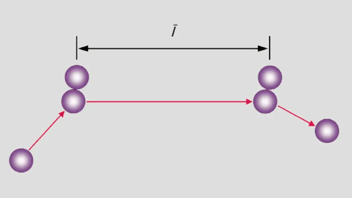
Figure 1-4: Mean free path between two collisions

For collisions of identical particles, the following applies for the mean free path:
Formula 1-11: Mean free path
- 𝑙¯ Mean free path [m]
- 𝑑𝑚 Molecular diameter [m]
- 𝑚 Mass [kg]
From Formula 1-11 it can be seen that the mean free path displays linear proportionality to the temperature and inverse proportionality to the pressure and molecular diameter. At this point we will disregard the further variants of this equation discussed in academic literature which examine issues such as collisions between different gas particles, collisions of gas particles with ions or electrons, and temperature effects.
To demonstrate the temperature dependence of the mean free path, Formula 1-11 is often written with the temperature as the only variable on the right-hand side of the equation:
Formula 1-11: Mean free path II
Table 1.5 shows the
\bar{l}\cdot p values for a number of selected gases at 0°C.
Gas | Chemical Symbol | 𝑙¯⋅𝑝 [m hPa] | 𝑙¯⋅𝑝 [m Pa] |
|---|---|---|---|
Hydrogen | H2 | 11.5·10-5 | 11.5·10-3 |
Nitrogen | N2 | 5.9·10-5 | 5.9·10-3 |
Oxygen | O2 | 6.5·10-5 | 6.5·10-3 |
Helium | He | 17.5·10-5 | 17.5·10-3 |
Neon | Ne | 12.7·10-5 | 12.7·10-3 |
Argon | Ar | 6.4·10-5 | 6.4·10-3 |
Air | 6.7·10-5 | 6.7·10-3 | |
Krypton | Kr | 4.9·10-5 | 4.9·10-3 |
Xenon | Xe | 3.6·10-5 | 3.6·10-3 |
Mercury | Hg | 3.1·10-5 | 3.1·10-3 |
Water vapor | H2O | 6.8·10-5 | 6.8·10-3 |
Carbon monoxide | CO | 6.8·10-5 | 6.0·10-3 |
Carbon dioxide | CO2 | 4.0·10-5 | 4.0·10-3 |
Hydrogen chloride | HCl | 3.3·10-5 | 3.3·10-3 |
Ammonia | NH3 | 3.2·10-5 | 3.2·10-3 |
Chlorine | Cl2 | 2.1·10-5 | 2.1·10-3 |
Table 1.5: Mean free path of selected gases at 273.15K [10]
Using the values from Table 1.5 we now estimate the mean free path of a nitrogen molecule at various pressures:
Pressure [Pa] | Pressure [hPa] | Mean free path [m] |
|---|---|---|
1·105 | 1·103 | 5.9·10-8 |
1·104 | 1·102 | 5.9·10-7 |
1·103 | 1·101 | 5.9·10-6 |
1·102 | 1·100 | 5.9·10-5 |
1·101 | 1·10-1 | 5.9·10-4 |
1·100 | 1·10-2 | 5.9·10-3 |
1·10-1 | 1·10-3 | 5.9·10-2 |
1·10-2 | 1·10-4 | 5.9·10-1 |
1·10-3 | 1·10-5 | 5.9·100 |
1·10-4 | 1·10-6 | 5.9·101 |
1·10-5 | 1·10-7 | 5.9·102 |
1·10-6 | 1·10-8 | 5.9·103 |
1·10-7 | 1·10-9 | 5.9·104 |
1·10-8 | 1·10-10 | 5.9·105 |
1·10-9 | 1·10-11 | 5.9·106 |
1·10-10 | 1·10-12 | 5.9·107 |
Table 1.6: Mean free path of a nitrogen molecule at 273.15K (0°C)
At atmospheric pressure a nitrogen molecule therefore travels a distance of 59 nm between two collisions, while at ultra-high vacuum at pressures below 10-8 hPa it travels a distance of several kilometers. The relation between molecular number density and the mean free path is shown in a graph in Figure 1.5.
-
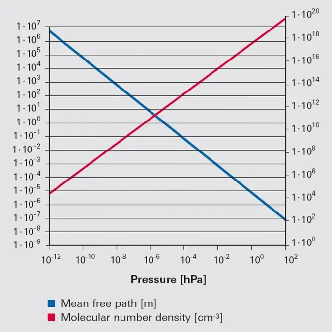
Figure 1.5: Molecular number density (red, right-hand y axis) and mean free path (blue, left-hand y axis) for nitrogen at a temperature of 273.15 K

1.2.6 Types of flow
The ratio of the mean free path to the flow channel diameter can be used to describe types of flow. This ratio is referred to as the Knudsen number:Formula 1-13: Knudsen number
-
\bar{l} Mean free path [m] -
d Diameter of flow channel [m] -
Kn Knudsen number dimensionless
The value of the Knudsen number characterizes the type of gas flow and assigns it to a particular pressure range. Table 1.7 gives an overview of the various types of flow in vacuum technology and their significant characterization parameters.
Profiles of the various types of flow regimes are shown in Figure 1.6.
-
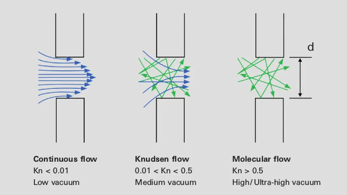
Figure 1.6: Profiles of the various types of flow regimes

Viscous flow in low vacuum
In viscous flow, also known as continuous flow, there are frequent collisions between gas molecules, but less frequently with the walls of the vessel. In this case, the mean free path of the gas molecules is significantly shorter than the dimensions of the flow channel.In the case of viscous flow, a distinction is made between laminar and turbulent flow. In laminar, or layered, flow the gas particles remain in the same displaced layers that are constantly parallel to each other. If the flow velocity increases, these layers are broken up and the fluid particles run into each other in a completely disordered way. This is termed turbulent flow. The boundary between these two areas of viscous flow can be expressed by the Reynolds number:
Formula 1-14: Reynolds number
- Re Reynolds number dimension less
- 𝜌 Density of the liquid [kg m-3]
- 𝜈 Mean velocity of the flow [m s-1]
- 𝑙 Characteristic length [m]
- 𝜂 Dynamic viscosity [Pa s]
Up to values of Re < 2,300 the flow will be laminar, and where Re > 4,000 the flow will be turbulent. In the range between 2,300 < Re < 4,000, the flow is predominantly turbulent. Laminar flow is also possible, however, both types of flow being unstable in this range.
Turbulent flow in a vacuum only occurs during pump-down operations from atmospheric pressure or when rapid venting is carried out. In vacuum systems, the pipes are dimensioned in such a manner that turbulent flow occurs only briefly at relatively high pressures, as the high flow resistance that occurs in this process necessitates that the pumps used produce higher volume flow rates.
Knudsen flow in medium vacuum
If the Knudsen number is between 0.01 and 0.5, this is termed Knudsen flow. Since many process pressures are in the medium vacuum range, this type of flow occurs with corresponding frequency.Molecular flow in high vacuum and ultra-high vacuum
At Knudsen numbers of 𝐾𝑛 > 0.5 molecular interaction virtually no longer occurs. What prevails is molecular flow. In this case, the mean free path is significantly greater than the diameter of the flow channel. In molecular flow, the product of pressure and component diameter is approximately ≤ 1.3 · 10-2 hPa cm. A graph showing an overview of flow ranges as a function of the product of pressure and component diameter is displayed in Figure 1.7.-
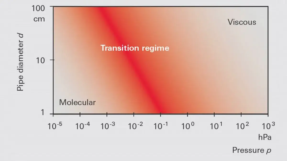
Figure 1.7: Flow ranges in vacuum as a function of p · d

This graph clearly shows that the classification, also found in Table 1.7, into vacuum ranges purely according to pressure is an inadmissible simplification. Since this classification is still in common usage, however, it is cited here.
Viscous flow | Knudsen flow | Molecular flow | |
|---|---|---|---|
Low vacuum | Medium vacuum | High / Ultra-high vacuum | |
Pressure range [hPa] | 103…1 | 1…10-3 | < 10-3 bzw. < 10-7 |
Pressure range [Pa] | 105…10 2 | 102…10 -1 | < 10-1 bzw. < 10-5 |
Knudsen number | Kn < 0.01 | 0.01 < Kn < 0.5 | Kn > 0.5 |
Reynolds number | Re < 2,300: laminar Re > 4,000: turbulent | ||
p · d [hPa cm] | p · d > 0.6 | 0.6 > p · d > 0.01 | p · d < 0.01 |
Table 1.7: Overview of types of flow regimes
1.2.7 pV throughput
Dividing the general gas equation (Formula 1-6) by time t obtains the gas flowFormula 1-15: pV throughput
𝑞𝑝𝑉pV through put [Pa m3 s-1]
As can be seen from the right-hand side of the equation, a constant mass flow is displaced at constant temperature T. This is also referred to as pV flow or gas throughput. Throughput is the gas flow rate transported by a vacuum pump.
As can be seen from the right-hand side of the equation, a constant mass flow is displaced at constant temperature T. This is also referred to as pV flow or gas throughput. Throughput is the gas flow rate transported by a vacuum pump.
Formula 1-16: Throughput of a vacuum pump
Dividing the throughput by the inlet pressure obtains a volume flow rate, the pumping speed of a vacuum pump:
Formula 1-17: Volume flow rate, or pumping speed, of a vacuum pump
A conversion table for various units of throughput is given in Table 1.8.
Pa m3 / s = W | mbar l / s | Torr l / s | atm cm3 / s | lusec | sccm | slm | Mol / s | |
|---|---|---|---|---|---|---|---|---|
Pa m3 / s | 1 | 10 | 7.5 | 9.87 | 7.5·103 | 592 | 0.592 | 4.41·10-4 |
mbar l / s | 0.1 | 1 | 0.75 | 0.987 | 750 | 59.2 | 5.92·10-2 | 4.41·10-5 |
Torr l / s | 0.133 | 1.33 | 1 | 1.32 | 1,000 | 78.9 | 7.89·10-2 | 5.85·10-5 |
atm cm3 / s | 0.101 | 1.01 | 0.76 | 1 | 760 | 59.8 | 5.98·10-2 | 4.45·10-5 |
lusec | 1.33·10-4 | 1.33·10-3 | 10-3 | 1.32·10-3 | 1 | 7.89·10-2 | 7.89·10-5 | 5.86·10-8 |
sccm | 1.69·10-3 | 1.69·10-2 | 1.27·10-2 | 1.67·10-2 | 12.7 | 1 | 10-3 | 7.45·10-7 |
slm | 1.69 | 16.9 | 12.7 | 16.7 | 1.27·104 | 1,000 | 1 | 7.45·10-4 |
Mol / s | 2.27·103 | 2.27·104 | 1.7·104 | 2.24·104 | 1.7·107 | 1.34·106 | 1.34·103 | 1 |
Table 1.8: Conversion table for units of throughput
1.2.8 Conductance
Generally speaking, vacuum chambers are connected to a vacuum pump via piping. Flow resistance occurs as a result of external friction between gas molecules and the wall surface and internal friction between the gas molecules themselves (viscosity). This flow resistance manifests itself in the form of pressure differences and volume flow rate, or pumping speed, losses. In vacuum technology, it is customary to use the reciprocal, the conductivity of piping 𝐿 or 𝐶 (conductance) instead of flow resistance 𝑊. The conductivity has the dimension of a volume flow rate and is normally expressed in [l s-1] or [m3 h-1].Gas flowing through piping produces a pressure differential Δ𝑝 at the ends of the piping. The following equation applies:
Formula 1-18: Definition of conductance
This principle is formally analogous to Ohm’s law of electrotechnology:
Formula 1-19: Ohm’s law
In a formal comparison of Formula 1-18 with Formula 1-19 𝑞𝑝𝑉 represents flow 𝐼, 𝐶 the reciprocal of resistance 1/𝑅 and Δ𝑝 the voltage 𝑈. If the components are connected in parallel, the individual conductivities are added:
Formula 1-20: Parallel connection conductance
and if connected in series, the resistances, i. e. the reciprocals, are added together:
Formula 1-21: Series connection conductivities
The conductance of pipes and pipe bends will differ in the various flow regimes. In viscous flow they are proportional to the mean pressure
\bar{p} and in molecular flow they are independent of pressure. Knudsen flow represents a transition between the two types of flow, and the conductivities vary with the Knudsen number.
-
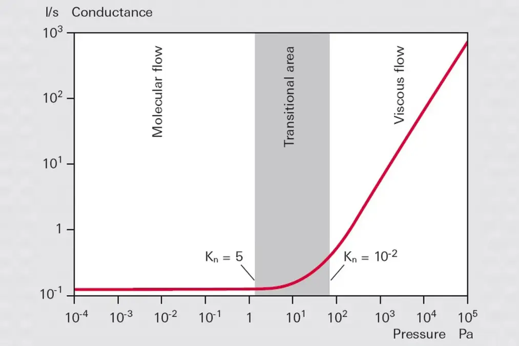
Figure 1.8: Conductance of a smooth round pipe as a function of the mean pressure in the pipe

A simple approximation for the Knudsen range can be obtained by adding the laminar and molecular conductivities. We would refer you to special literature for exact calculations of the conductance still in the laminar flow range and already in the molecular flow range as well as conductance calculations taking into account inhomogeneities at the inlet of a pipe.
This publication is restricted to the consideration of the conductivities of orifices and long, round pipes for laminar and molecular flow ranges.
Orifices are frequently flow resistances in vacuum systems. Examples of these are constrictions in the cross-section of valves, ventilation devices or orifices in measuring domes for measuring the pumping speed. In pipe openings in vessel walls the orifice resistance of the inlet opening must also be taken into account in addition to the pipe resistance.
Choked flow
Let us consider the venting of a vacuum chamber. When the venting valve is opened, ambient air flows into the vessel at high velocity at a pressure of p. The flow velocity reaches not more than sonic velocity. If the gas has reached sonic velocity, the maximum gas throughput has also been reached at which the vessel can be vented. The throughput flowing through it 𝑞𝑝𝑉 is not a function of the vessel’s interior pressure 𝑝𝑖. The following applies for air:Formula 1-22: Blocking of an orifice
- 𝑑 Diameter of orifice [cm]
- 𝑝𝑎 External pressure on the vessel [hPa]
Gas dynamic flow
If the pressure in the vessel now rises beyond a critical pressure, gas flow is reduced and we can use gas dynamic laws according to Bernoulli and Poiseuille to calculate it. The immersive gas flow 𝑞𝑝𝑉 and the conductance are dependent on- Narrowest cross-section of the orifice
- External pressure on the vessel
- Internal pressure in the vessel
- Universal gas constant
- Absolute temperature
- Molar mass
- Adiabatic exponent (= ratio of specific or molar heat capacities at constant pressure 𝑐𝑝 or constant volume 𝑐𝑉)
Molecular flow
If an orifice connects two vessels in which molecular flow conditions exist (i.e. if the mean free path is considerably greater than the diameter of the vessel), the following will apply for the displaced gas quantity 𝑞𝑝𝑉 per unit of timeFormula 1-23: Orifice flow
- 𝐴 Cross-section of orifice [m2]
- 𝑐¯ Mean thermal velocity [m s-1]
According to Formula 1-23 the following applies for the orifice conductivity
Formula 1-24: Orifice conductivity
- 𝑘 Boltzmann constant [m2 kg s-2 K-1]
- 𝑚 0Molecular mass in kg
For air with a temperature of 293 K we obtain
Formula 1-25: Orifice conductivity for air in [l / s]
- 𝐴 Cross-section of orifice [cm2]
- 𝐶 Conductivity [l s-1]
This formula can be used to determine the maximum possible pumping speed of a vacuum pump with an inlet port A. The maximum pumping speed of a pump under molecular flow conditions is therefore determined by the inlet port.
Let us now consider specific pipe conductivities. In the case of laminar flow, the conductivity of a pipe is proportional to the mean pressure:
Formula 1-26: Conductance of a pipe in laminar flow
Physical sign | unit |
|---|---|
[Pa
| |
d | [m] |
l | [m] |
p | [Pa] |
C | [m3/s] |
For air at 20°C we obtain
Formula 1-27: Conductance of a pipe in laminar flow for air
- l Length of pipe [cm]
- d Diameter of pipe [cm]
-
\bar{p} Pressure [Pa] - C Conductivity [l s-1]
In the molecular flow regime, conductance is constant and is not a function of pressure. It can be considered to be the product of the orifice conductivity of the pipe opening
Formula 1-28: Molecular pipe flow
The mean probability 𝑃pipe,mol can be calculated with a computer program for different pipe profiles, bends or valves using a Monte Carlo simulation. In this connection, the trajectories of individual gas molecules through the component can be tracked on the basis of wall collisions.
The following applies for long round pipes:
The following applies for long round pipes:
Formula 1-29: Passage probability for long round pipes
If we multiply this value by the orifice conductivity (Formula 1-24), we obtain
Formula 1-30: Molecular pipe conductivity
For air at 20°C we obtain
Formula 1-31: Molecular pipe conductivity
𝑙 Length of pipe [cm]
𝑑 Diameter of pipe [cm]
𝐶 Conductivity [l s-1]
𝑑 Diameter of pipe [cm]
𝐶 Conductivity [l s-1]